| id | job | price_glass |
|---|---|---|
| 1 | Student | 0 |
| 2 | Retired | 0 |
| 3 | Other | 0 |
| 4 | Employed | 10 |
| 5 | Employed | See comment |
| 6 | Student | 05-Oct |
| 7 | Student | 0 |
| 8 | Retired | 0 |
| 9 | Student | 10 |
| 10 | Employed | 0 |
| 11 | Employed | 20 (2chf per person with 10 people in the WG) |
| 12 | Student | 10 |
| 13 | Student | 10 |
| 14 | Employed | 0 |
| 15 | Student | 10 |
| 16 | Student | 0 |
| 17 | Employed | 5 to 10 |
| 18 | Other | 0 |
| 19 | Student | 0 |
| 20 | Employed | 10 |
| 21 | Employed | 0 |
| 22 | Employed | 5 |
Concept of tidy data, vectors and pivoting
CVEN 5999 - Summer 2025
Lars Schöbitz
Learning Objectives (for this week)
- Learners can apply functions from the dplyr R Package to transform their data from a wide to a long format and vice versa.
- Learners can list the four main atomic vector types in R.
- Learners can explain the three characteristics of tidy data.
Part 1: Data types and vectors
Why care about data types?
Example: survey data
Data from: (Ben Aleya et al. 2022)
Oh why won’t you work?!
Oh why won’t you still work??!!
Take a breath and look at your data
| id | job | price_glass |
|---|---|---|
| 1 | Student | 0 |
| 2 | Retired | 0 |
| 3 | Other | 0 |
| 4 | Employed | 10 |
| 5 | Employed | See comment |
| 6 | Student | 05-Oct |
| 7 | Student | 0 |
| 8 | Retired | 0 |
| 9 | Student | 10 |
| 10 | Employed | 0 |
| 11 | Employed | 20 (2chf per person with 10 people in the WG) |
| 12 | Student | 10 |
| 13 | Student | 10 |
| 14 | Employed | 0 |
| 15 | Student | 10 |
| 16 | Student | 0 |
| 17 | Employed | 5 to 10 |
| 18 | Other | 0 |
| 19 | Student | 0 |
| 20 | Employed | 10 |
| 21 | Employed | 0 |
| 22 | Employed | 5 |
Very common data tidying step!
Very common data tidying step!
| id | job | price_glass_new | price_glass |
|---|---|---|---|
| 1 | Student | 0 | 0 |
| 2 | Retired | 0 | 0 |
| 3 | Other | 0 | 0 |
| 4 | Employed | 10 | 10 |
| 5 | Employed | NA | See comment |
| 6 | Student | 7.5 | 05-Oct |
| 7 | Student | 0 | 0 |
| 8 | Retired | 0 | 0 |
| 9 | Student | 10 | 10 |
| 10 | Employed | 0 | 0 |
| 11 | Employed | 20 | 20 (2chf per person with 10 people in the WG) |
| 12 | Student | 10 | 10 |
| 13 | Student | 10 | 10 |
| 14 | Employed | 0 | 0 |
| 15 | Student | 10 | 10 |
| 16 | Student | 0 | 0 |
| 17 | Employed | 7.5 | 5 to 10 |
| 18 | Other | 0 | 0 |
| 19 | Student | 0 | 0 |
| 20 | Employed | 10 | 10 |
| 21 | Employed | 0 | 0 |
| 22 | Employed | 5 | 5 |
Sumamrise? Argh!!!!
survey_data_small |>
  mutate(price_glass_new = case_when(
    price_glass == "5 to 10" ~ "7.5",
    price_glass == "05-Oct" ~ "7.5",
    str_detect(price_glass, pattern = "20") == TRUE ~ "20",
    str_detect(price_glass, pattern = "See comment") == TRUE ~ NA_character_,
    TRUE ~ price_glass
  )) |>
  summarise(mean_price_glass = mean(price_glass_new, na.rm = TRUE))
# A tibble: 1 × 1
mean_price_glass
<dbl>
1 NAAlways respect your data types!
Taking the mean of vector with type “character” is not possible.
# A tibble: 22 × 4
      id job      price_glass price_glass_new
   <int> <chr>    <chr>       <chr>
 1     1 Student  0           0
 2     2 Retired  0           0
 3     3 Other    0           0
 4     4 Employed 10          10
 5     5 Employed See comment <NA>
 6     6 Student  05-Oct      7.5
 7     7 Student  0           0
 8     8 Retired  0           0
 9     9 Student  10          10
10    10 Employed 0           0
# ℹ 12 more rows
Always respect your data types!
survey_data_small |>
  mutate(price_glass_new = case_when(
    price_glass == "5 to 10" ~ "7.5",
    price_glass == "05-Oct" ~ "7.5",
    str_detect(price_glass, pattern = "20") == TRUE ~ "20",
    str_detect(price_glass, pattern = "See comment") == TRUE ~ NA_character_,
    TRUE ~ price_glass
  )) |>
  mutate(price_glass_new = as.numeric(price_glass_new)) |>
  summarise(mean_price_glass = mean(price_glass_new, na.rm = TRUE))
# A tibble: 1 × 1
mean_price_glass
<dbl>
1 4.76Live Coding Exercise: Vectors
wk-05 repository
Follow along on the screen
- Open the GitHub organisation for the course: https://github.com/cven5999-ss25
- You will find a repository titled: wk-05-USERNAME (with your GitHub Username)
- You will “clone” this repository to Posit Cloud
Break

10:00
Part 2: tidyr - long and wide formats
.
.
.
A grammar of data tidying
The goal of tidyr is to help you tidy your data via
- pivoting for going between wide and long data
- splitting and combining character columns
- nesting and unnesting columns
- clarifying how
NAs should be treated
Pivoting data
Waste characterisation data
| objid | location | pet | metal_alu | glass | paper | other | total |
|---|---|---|---|---|---|---|---|
| 900 | eth | 0.06 | 0.06 | 0.58 | 0.21 | 1.14 | 2.05 |
| 899 | eth | 0.14 | 0.01 | 0.18 | 0.28 | 3.04 | 3.64 |
| 921 | old_town | 0.00 | 0.00 | 0.00 | 0.41 | 1.57 | 1.99 |
| 916 | old_town | 0.17 | 0.04 | 0.80 | 0.55 | 0.62 | 2.19 |
| 900 | eth | 0.10 | 0.04 | 0.00 | 0.40 | 0.58 | 1.12 |
| 899 | eth | 0.08 | 0.03 | 0.00 | 0.05 | 0.34 | 0.50 |
| 921 | old_town | 0.08 | 0.03 | 0.30 | 0.40 | 1.52 | 2.33 |
| 916 | old_town | 0.11 | 0.04 | 0.92 | 1.01 | 1.99 | 4.07 |
How would you plot this?

Three variables
| objid | location | total |
|---|---|---|
| 900 | eth | 2.05 |
| 899 | eth | 3.64 |
| 921 | old_town | 1.99 |
| 916 | old_town | 2.19 |
| 900 | eth | 1.12 |
| 899 | eth | 0.50 |
| 921 | old_town | 2.33 |
| 916 | old_town | 4.07 |
Three variables -> three aesthetics

And how to plot this?

Reminder: Data (in wide format)
| objid | location | pet | metal_alu | glass | paper | other |
|---|---|---|---|---|---|---|
| 900 | eth | 0.06 | 0.06 | 0.58 | 0.21 | 1.14 |
| 899 | eth | 0.14 | 0.01 | 0.18 | 0.28 | 3.04 |
| 921 | old_town | 0.00 | 0.00 | 0.00 | 0.41 | 1.57 |
| 916 | old_town | 0.17 | 0.04 | 0.80 | 0.55 | 0.62 |
| 900 | eth | 0.10 | 0.04 | 0.00 | 0.40 | 0.58 |
| 899 | eth | 0.08 | 0.03 | 0.00 | 0.05 | 0.34 |
| 921 | old_town | 0.08 | 0.03 | 0.30 | 0.40 | 1.52 |
| 916 | old_town | 0.11 | 0.04 | 0.92 | 1.01 | 1.99 |
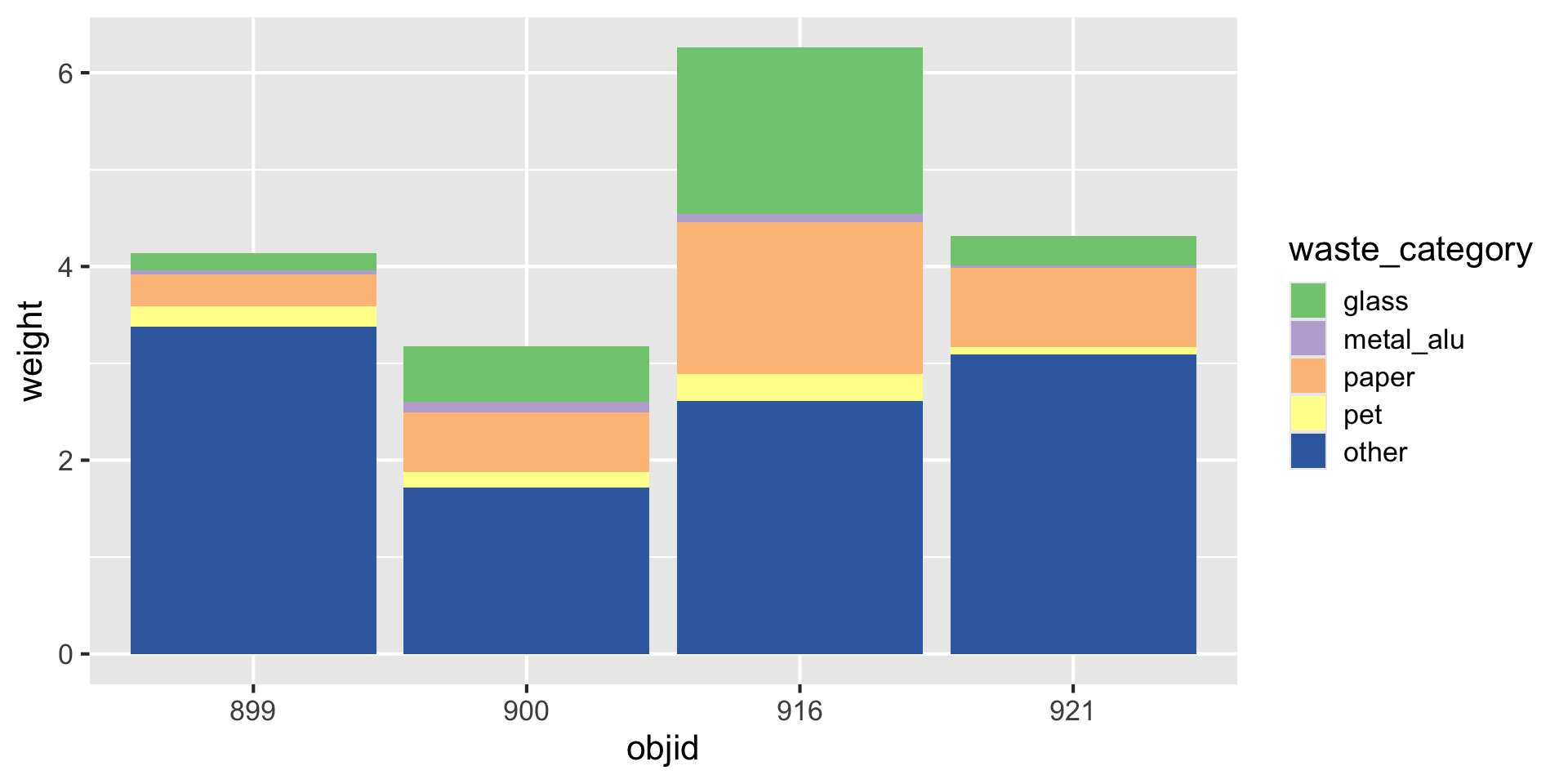
You need: A long format
| objid | location | waste_category | weight |
|---|---|---|---|
| 900 | eth | pet | 0.06 |
| 900 | eth | metal_alu | 0.06 |
| 900 | eth | glass | 0.58 |
| 900 | eth | paper | 0.21 |
| 900 | eth | other | 1.14 |
| 899 | eth | pet | 0.14 |
| 899 | eth | metal_alu | 0.01 |
| 899 | eth | glass | 0.18 |
| 899 | eth | paper | 0.28 |
| 899 | eth | other | 3.04 |
| 921 | old_town | pet | 0.00 |
| 921 | old_town | metal_alu | 0.00 |
| 921 | old_town | glass | 0.00 |
| 921 | old_town | paper | 0.41 |
| 921 | old_town | other | 1.57 |
| 916 | old_town | pet | 0.17 |
| 916 | old_town | metal_alu | 0.04 |
| 916 | old_town | glass | 0.80 |
| 916 | old_town | paper | 0.55 |
| 916 | old_town | other | 0.62 |
| 900 | eth | pet | 0.10 |
| 900 | eth | metal_alu | 0.04 |
| 900 | eth | glass | 0.00 |
| 900 | eth | paper | 0.40 |
| 900 | eth | other | 0.58 |
| 899 | eth | pet | 0.08 |
| 899 | eth | metal_alu | 0.03 |
| 899 | eth | glass | 0.00 |
| 899 | eth | paper | 0.05 |
| 899 | eth | other | 0.34 |
| 921 | old_town | pet | 0.08 |
| 921 | old_town | metal_alu | 0.03 |
| 921 | old_town | glass | 0.30 |
| 921 | old_town | paper | 0.40 |
| 921 | old_town | other | 1.52 |
| 916 | old_town | pet | 0.11 |
| 916 | old_town | metal_alu | 0.04 |
| 916 | old_town | glass | 0.92 |
| 916 | old_town | paper | 1.01 |
| 916 | old_town | other | 1.99 |
Three variables -> three aesthetics
How to
| objid | location | pet | metal_alu | glass | paper | other |
|---|---|---|---|---|---|---|
| 900 | eth | 0.06 | 0.06 | 0.58 | 0.21 | 1.14 |
| 899 | eth | 0.14 | 0.01 | 0.18 | 0.28 | 3.04 |
| 921 | old_town | 0.00 | 0.00 | 0.00 | 0.41 | 1.57 |
| 916 | old_town | 0.17 | 0.04 | 0.80 | 0.55 | 0.62 |
| 900 | eth | 0.10 | 0.04 | 0.00 | 0.40 | 0.58 |
| 899 | eth | 0.08 | 0.03 | 0.00 | 0.05 | 0.34 |
| 921 | old_town | 0.08 | 0.03 | 0.30 | 0.40 | 1.52 |
| 916 | old_town | 0.11 | 0.04 | 0.92 | 1.01 | 1.99 |
How to
| objid | location | waste_category | weight |
|---|---|---|---|
| 900 | eth | pet | 0.06 |
| 900 | eth | metal_alu | 0.06 |
| 900 | eth | glass | 0.58 |
| 900 | eth | paper | 0.21 |
| 900 | eth | other | 1.14 |
| 899 | eth | pet | 0.14 |
| 899 | eth | metal_alu | 0.01 |
| 899 | eth | glass | 0.18 |
| 899 | eth | paper | 0.28 |
| 899 | eth | other | 3.04 |
| 921 | old_town | pet | 0.00 |
| 921 | old_town | metal_alu | 0.00 |
| 921 | old_town | glass | 0.00 |
| 921 | old_town | paper | 0.41 |
| 921 | old_town | other | 1.57 |
| 916 | old_town | pet | 0.17 |
| 916 | old_town | metal_alu | 0.04 |
| 916 | old_town | glass | 0.80 |
| 916 | old_town | paper | 0.55 |
| 916 | old_town | other | 0.62 |
| 900 | eth | pet | 0.10 |
| 900 | eth | metal_alu | 0.04 |
| 900 | eth | glass | 0.00 |
| 900 | eth | paper | 0.40 |
| 900 | eth | other | 0.58 |
| 899 | eth | pet | 0.08 |
| 899 | eth | metal_alu | 0.03 |
| 899 | eth | glass | 0.00 |
| 899 | eth | paper | 0.05 |
| 899 | eth | other | 0.34 |
| 921 | old_town | pet | 0.08 |
| 921 | old_town | metal_alu | 0.03 |
| 921 | old_town | glass | 0.30 |
| 921 | old_town | paper | 0.40 |
| 921 | old_town | other | 1.52 |
| 916 | old_town | pet | 0.11 |
| 916 | old_town | metal_alu | 0.04 |
| 916 | old_town | glass | 0.92 |
| 916 | old_town | paper | 1.01 |
| 916 | old_town | other | 1.99 |
Three variables -> three aesthetics

Live Coding Exercise: Pivoting
live-tidyr-pivoting
- Head over to posit.cloud
- Open the workspace for the course cven5999-ss25
- Open “Content”
- Open your project
- Follow along with me
Homework week 5
Homework due dates
- All material on course website
- Homework assignment & learning reflection due: 2025-07-04
Thanks! 🌻
Slides created via revealjs and Quarto: https://quarto.org/docs/presentations/revealjs/
Access slides as PDF on GitHub
All material is licensed under Creative Commons Attribution Share Alike 4.0 International.
References
Ben Aleya, Ali, Daniel Biek, Lin Boynton, Julia Jaeggi, Sebastian Camilo Loos, Chiara Meyer-Piening, Jonathan Olal Ogwang, et al. 2022. “Research Beyond the Lab, Spring Term 2022, Global Health Engineering, ETH Zurich. Raw Data and Analysis-Ready Derived Data on Waste Management in Public Spaces in Zurich, Switzerland.” Zenodo. https://doi.org/10.5281/ZENODO.7331119.